Tutorial 1: Kernel1D

import matplotlib.pyplot as plt
import torch
from spectpsftoolbox.kernel1d import FunctionKernel1D, ArbitraryKernel1D
from spectpsftoolbox.operator2d import GaussianOperator
device = torch.device('cuda' if torch.cuda.is_available() else 'cpu')

1D kernels in spectpsftoolbox can be expressed as

\[f(x,a) = A(a,\vec{b}) \cdot k\left(\frac{x}{\sigma(a,\vec{b})}\right)\]

where \(x\) is position and \(a\) is some scalar that the kernel depends on, and \(\vec{b}\) are additional hyperparameters. The amplitude \(A(a)\) and scaling \(\sigma(a)\) may also depend on additional parameters. We start be defining them:

• \(A(a,\vec{b}) = b_0 e^{-b_1a}\)

• \(\sigma(a,\vec{b}) = b_0(a+0.1)\)

amplitude_fn = lambda a, bs: bs[0]*torch.exp(-bs[1]*a)
sigma_fn = lambda a, bs: bs[0]*(a+0.1)

Now we define the initial parameters \(\vec{b}\) they are expected to be torch tensors:

• In the code below, we initialize \(b_0=2\) and \(b_1=0.1\) for \(A(a,\vec{b})\)

amplitude_params = torch.tensor([2,0.1], device=device, dtype=torch.float32)
sigma_params = torch.tensor([0.3], device=device, dtype=torch.float32)

Function Kernel

For function kernels, \(k(x)\) is set explicitly. Let’s set \(k(x) = e^{-|x|}\)

kernel_fn = lambda x: torch.exp(-torch.abs(x))

Now we can build the function kernel:

kernel1D = FunctionKernel1D(kernel_fn, amplitude_fn, sigma_fn, amplitude_params, sigma_params)

/data/anaconda/envs/pytomo_install_test/lib/python3.11/site-packages/torchquad/integration/utils.py:255: UserWarning: DEPRECATION WARNING: In future versions of torchquad, an array-like object will be returned.
  warnings.warn(

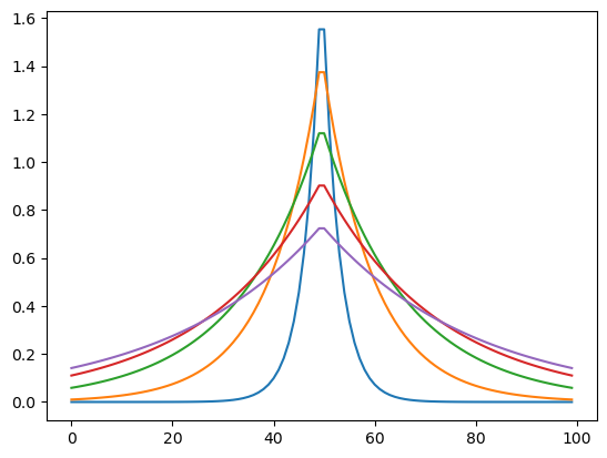
Lets look at the value of the kernel at various values of \(a\):

x = torch.linspace(-5,5,100).to(device)
a = torch.linspace(1,10,5).to(device)

kernel_value = kernel1D(x, a)

plt.plot(kernel_value.cpu().T)
plt.show()

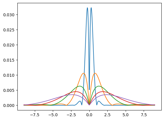
We can also get normalized values:

kernel_value = kernel1D(x, a, normalize=True)
print(kernel_value.sum(dim=1))
plt.plot(kernel_value.cpu().T)
plt.show()

tensor([0.9961, 0.9930, 0.9504, 0.8828, 0.8111], device='cuda:0')

Arbitrary Kernels

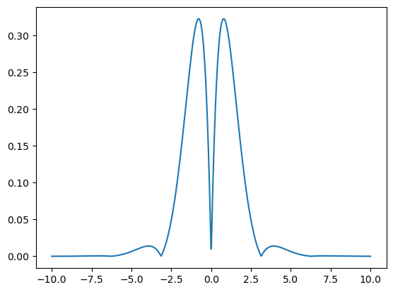
We can also define arbitrary kernels that have no explicit functional form given some data. For suppose the below was data we collected:

x = torch.linspace(-10,10,1000).to(device)
k_data = torch.exp(-torch.abs(x))*torch.abs(torch.sin(x))
plt.plot(x.cpu(),k_data.cpu())

[<matplotlib.lines.Line2D at 0x7f6cdc9c8110>]

Then we can define an arbitrary kernel:

arb_kernel1D = ArbitraryKernel1D(
    kernel=k_data,
    amplitude_fn=amplitude_fn,
    sigma_fn=sigma_fn,
    amplitude_params=amplitude_params,
    sigma_params=sigma_params,
    dx0 = x[1]-x[0] # needs to be provided
)

Lets define some new positions different from the above and evaluate the kernel:

x = torch.linspace(-9,9,500).to(device)
a = torch.linspace(1,10,5).to(device)
kernel_value = arb_kernel1D(x, a)

plt.plot(x.cpu(), kernel_value.cpu().T)
plt.show()

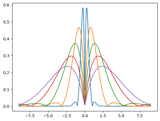
We can also get normalized values (each sums to 1)

• Some of the more stretched ones don’t sum to 1 because they have non-zero values outside the field of view

kernel_value = arb_kernel1D(x, a, normalize=True)
print(kernel_value.sum(dim=1))
plt.plot(x.cpu(), kernel_value.cpu().T)
plt.show()

tensor([1.0008, 1.0000, 0.9956, 0.9684, 0.9556], device='cuda:0')