Tutorial 8: Lu177 Low Energy Collimator Modeling#

[1]:

import matplotlib.pyplot as plt
import torch
import numpy as np
import pytomography
from pytomography.io.SPECT import simind
from pytomography.projectors.SPECT import SPECTSystemMatrix
from pytomography.transforms.SPECT import SPECTAttenuationTransform, SPECTPSFTransform
from pytomography.algorithms import OSEM
from pytomography.likelihoods import PoissonLogLikelihood
from spectpsftoolbox.simind_io import get_projections, get_source_detector_distances
from pytomography.io.SPECT.shared import subsample_projections_and_modify_metadata, subsample_amap
from spectpsftoolbox.operator2d import NearestKernelOperator
device = pytomography.device


          -  -  -  -  -  -  -  -   -  -  -  -
          P  A  R  A  L  L  E  L | P  R  O  J
          -  -  -  -  -  -  -  -   -  -  -  -

    =================================================

         Please consider citing our publication
      ---------------------------------------------
      Georg Schramm and Kris Thielemans:
      "PARALLELPROJ—an open-source framework for
       fast calculation of projections in
       tomography"
      Front. Nucl. Med., 08 January 2024
      Sec. PET and SPECT, Vol 3
      https://doi.org/10.3389/fnume.2023.1324562

    =================================================

    parallelproj C    lib: /data/anaconda/envs/pytomo_install_test/lib/libparallelproj_c.so.1.8.0
    parallelproj CUDA lib: /data/anaconda/envs/pytomo_install_test/lib/libparallelproj_cuda.so.1.8.0

This tutorial looks at reconstructing Lu177 data acquired with a low energy (as opposed to a typical medium energy) collimator. First, we open some point source data of 208keV photons impinging on a medium energy collimator:

[2]:

headerpaths = np.array([f'/disk1/psf_data/208keV_LE_PSF/point_position{i}_tot_w1.h00' for i in range(538,1638)])
respaths = np.array([f'/disk1/psf_data/208keV_LE_PSF/point_position{i}.res' for i in range(538,1638)])
distances = get_source_detector_distances(respaths).to(device)
projectionss_data = get_projections(headerpaths).to(device)[:,1:,1:]

[3]:

fig, ax = plt.subplots(2,5,figsize=(10,4))
for i, IDX in enumerate([0,100,200,300,400,500,600,700,800,900]):
    plt.sca(ax.ravel()[i])
    plt.imshow(projectionss_data[IDX].cpu().numpy(), cmap='magma', vmax=projectionss_data[IDX].cpu().numpy().max()/10)
    plt.title(f'{distances[IDX].item():.0f}cm from scanner', fontsize=7)
    plt.axis('off')

../_images/tutorials_8_pytomography_lu177_le_recon_4_0.png

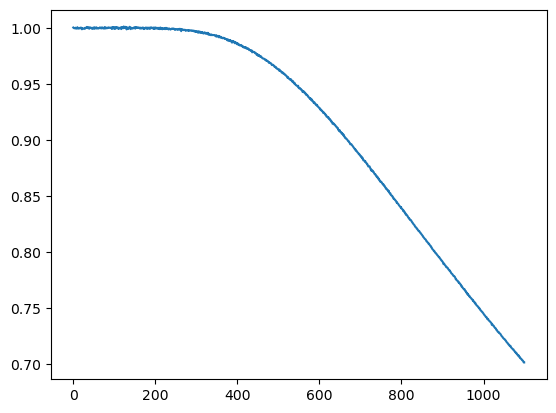
Let’s create a kernel out of this:

[4]:

projectionss_data /= projectionss_data[0:100].sum().reshape(-1,1,1) / 100
psf_operator = NearestKernelOperator(
    psf_data = projectionss_data,
    distances = distances,
    dr0 = (0.48,0.48)
)

[5]:

plt.plot(projectionss_data.sum(dim=(1,2)).cpu())

[5]:

[<matplotlib.lines.Line2D at 0x7fd699b7c990>]

../_images/tutorials_8_pytomography_lu177_le_recon_7_1.png

Let’s perform PyTomography reconstruction. We’ll get all the necessary data:

[6]:

activity = 1000 # MBq
dT = 15 # seconds per projection

paths = [f'/disk1/psf_data/208keV_LE_jaszak/tot_w{i}.h00' for i in range(1,4)]
object_meta, proj_meta = simind.get_metadata(paths[0])
projections = simind.get_projections(paths)
projections = torch.poisson(activity*dT*projections)

object_meta, proj_meta, projections = subsample_projections_and_modify_metadata(object_meta, proj_meta, projections, N_pixel = 2, N_angle=1)
photopeak = projections[1]
ww_peak = simind.get_energy_window_width(paths[1])
ww_lower = simind.get_energy_window_width(paths[0])
ww_upper = simind.get_energy_window_width(paths[2])
lower_scatter = projections[0]
upper_scatter = projections[2]
scatter = (lower_scatter/ww_lower+upper_scatter/ww_upper)*ww_peak/2
attenuation_path = '/disk1/psf_data/208keV_LE_jaszak/amap.hct'
attenuation_map = simind.get_attenuation_map(attenuation_path)
attenuation_map = subsample_amap(attenuation_map, 2)
att_transform = SPECTAttenuationTransform(attenuation_map)

We’ll reconstruct using OSEM(20it,8ss).

Reconstruction using standard PSF modeling:

[7]:

psf_meta = simind.get_psfmeta_from_header(paths[0])
psf_transform = SPECTPSFTransform(psf_meta)
system_matrix = SPECTSystemMatrix(
    obj2obj_transforms = [att_transform,psf_transform],
    proj2proj_transforms = [],
    object_meta = object_meta,
    proj_meta = proj_meta
    )
likelihood = PoissonLogLikelihood(system_matrix, projections[1], additive_term=scatter)
recon_algorithm = OSEM(likelihood)
recon_BASIC = recon_algorithm(n_iters = 40, n_subsets = 8)

Recon using Monte Carlo PSF:

[8]:

psf_transform = SPECTPSFTransform(psf_operator=psf_operator)
system_matrix = SPECTSystemMatrix(
    obj2obj_transforms = [att_transform,psf_transform],
    proj2proj_transforms = [],
    object_meta = object_meta,
    proj_meta = proj_meta
    )
likelihood = PoissonLogLikelihood(system_matrix, projections[1], additive_term=scatter)
recon_algorithm = OSEM(likelihood)
recon_MONTECARLO = recon_algorithm(n_iters = 40, n_subsets = 8)

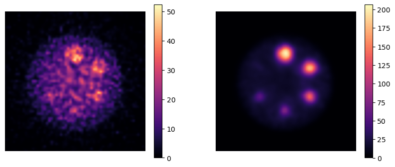
Compare the two:

[9]:

fig, ax = plt.subplots(1,2,figsize=(10,4))
plt.subplot(121)
plt.imshow(recon_BASIC[:,:,64].cpu().T, cmap='magma', interpolation='gaussian')
plt.xlim(64-30, 64+30)
plt.ylim(64-30, 64+30)
plt.colorbar()
plt.axis('off')
plt.subplot(122)
plt.imshow(recon_MONTECARLO[:,:,64].cpu().T, cmap='magma', interpolation='gaussian')
plt.xlim(64-30, 64+30)
plt.ylim(64-30, 64+30)
plt.colorbar()
plt.axis('off')

[9]:

(34.0, 94.0, 34.0, 94.0)

../_images/tutorials_8_pytomography_lu177_le_recon_15_1.png

[10]:

torch.save(recon_BASIC, '/disk1/psf_data/toolbox_plots_data/lu177_le_badPSF_40it8ss.pt')
torch.save(recon_MONTECARLO, '/disk1/psf_data/toolbox_plots_data/lu177_le_goodPSF_40it8ss.pt')

The one that uses the Monte Carlo kernels for PSF modeling is much better.

Tutorial 8: Lu177 Low Energy Collimator Modeling#

This Page